Emma Clinton's Portfolio
Collection of Open Source GIScience Projects
Project maintained by emmaclinton Hosted on GitHub Pages — Theme by mattgraham
RE- Replication of Rosgen Stream Classification
Replication of
A classification of natural rivers
Original study by Rosgen, D. L. in CATENA 22 (3):169–199. https://linkinghub.elsevier.com/retrieve/pii/0341816294900019.
and Replication by: Kasprak, A., N. Hough-Snee, T. Beechie, N. Bouwes, G. Brierley, R. Camp, K. Fryirs, H. Imaki, M. Jensen, G. O’Brien, D. Rosgen, and J. Wheaton. 2016. The Blurred Line between Form and Process: A Comparison of Stream Channel Classification Frameworks ed. J. A. Jones. PLOS ONE 11 (3):e0150293. https://dx.plos.org/10.1371/journal.pone.0150293.
Replication Authors: Emma Clinton, Zach Hilgendorf, Joseph Holler, and Peter Kedron.
Replication Materials Available at: RE-rosgen
Created: 21 March 2021
Revised: 24 March 2021
Abstract / Introduction
There is much appeal in developing and utilizing a standard and quantifiable method of stream classification. Standardizing the way streams are classified allows communication across disciplines regarding river systems and their predicted behaviors, their past behaviors, and the best ways in which to manage or restore them. The Rosgen Classification System (RCS), probably the most common method for stream classification in North America, is one such method of stream taxonomy. The RCS classifies streams based on physical metrics that are informed by empirical field data (Kasprak et al., 2016). The RCS involves classifying streams based on directly measurable variables, ranging from very broad to very reach-specific characteristics (Rosgen, 1994). Kasprak et al. (2016) attempted to replicate the RCS classification system, which is normally based on empirical field-based data, using geographic data and on a watershed scale.
Our replication study focuses on the first two levels of stream classifications: Level I and Level II. Level I is the “broad geomorphic characterization”, while Level II is the morphological description of a reach (Rosgen, 1994). Level I is based on longitudinal profile characteristics, cross-section morphology, and plan view morphology (stream pattern). Level II incorporates entrenchment (width of flood-prone area to bankfull surface width of channel), width/depth ratio (bankfull channel width / mean bankfull depth), sinuosity (ratio of stream length to valley length) and channel materials (Rosgen, 1994).
Kasprak et al. (2016) utilized the RCS to classify 33 reach stream types in the John Day River (located in Oregon in the Columbia River Valley). In this study, the researchers used DEM data and expert-generated ground-based assessment data in a GIS to assign a Level I and Level II classification to different reaches in the John Day River. Whereas Kasprak et al. (2016) used the River Bathymetry Toolkit, our study attempted to replicate the results of Kasprak et al. (2016) using open source GIS and statistical software (GRASS and R, respectively). We used CHaMP data from the Columbia Habitat Monitoring Program that was used in the Kasprak study in conjuction with DEM LiDAR data from the Camp Creek LiDAR Project (DEM data with a lower spatial resolution than that used in the original study) to extrapolate Level I and Level II classifications for a randomly assigned reach in the John Day River.
Variables
Level I Variables as defined by Rosgen (1994):
- Entrenchment: Measured as the width at 2x the bankfull depth divided by the bankfull width
- Width/Depth Ratio: Bankfull channel width divided by bankfull mean depth
- Sinuosity: Ratio of stream length to valley length
Level II Variables as defined by Rosgen (1994):
- Slope Range: Difference in water surface elevation per unit stream length
- Channel Material: The size and composition of channel materials in the stream (in our case, based on the fact that 50% of the substrate is of the same size class or finer than the class assigned)
Materials and Procedure
In this replication study, the open source software platforms GRASS and R were used to replicate the Rosgen river classification for a specific reach of the John Day River up to Level II. Note that in order to complete this analysis using MacOS, the software platforms The Unarchiver and XCode are required.
This replication study was an attempt to use Open Source GIS to replicate the methods of (Rosgen, 1994) and compare our results to those of the Rosgen (1994) replication by Kasprak et al. (2016). Kasprak et al. (2016) used different DEM data and software platforms (River Bathymetry Tool) than we used in our analysis. The scope of the analysis was also different in the original study, which looked at reaches on the watershed scale. Instead, we focused only on a single, randomly assigned reach. In this procedure, each member of the team was assigned a random study site that was used in the original experimental setup. Study sites came from the CHaMP datafile. This instance looks at the site with the loc_id of 7 (CBW05583-275954).
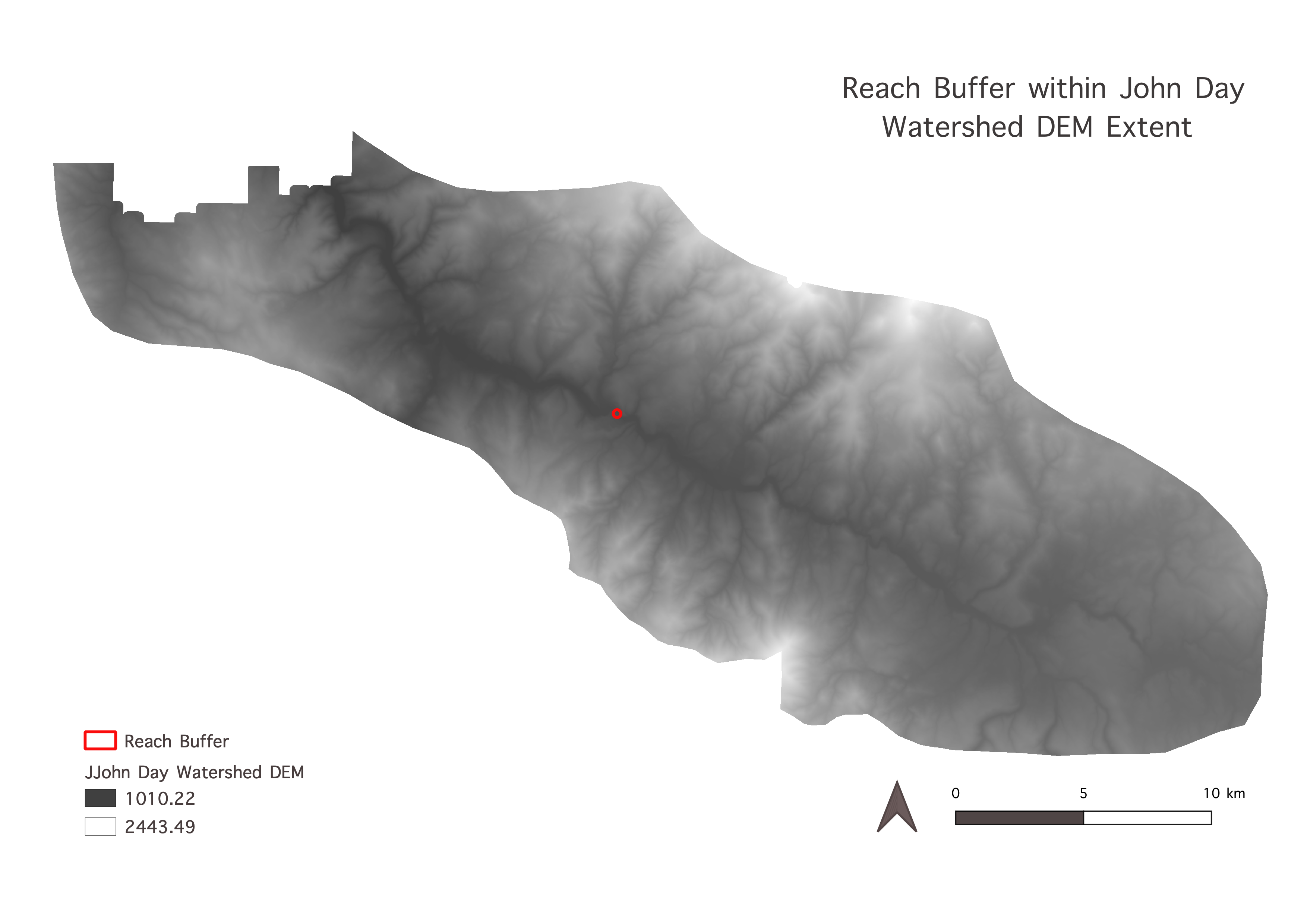 (Fig. 1) Randomly assigned sample point (CBW05583-275954).
The instructions for the work in GRASS can be found here. Finding the centerlines of the river reach and corresponding valley was completed in GRASS. The first step in this process was to define the “reach” area for the point assigned for study and preprocess/create our layers to use in our digitization process (Figs. 2a and 2b). To do this, we used this model, created by Joe Holler.
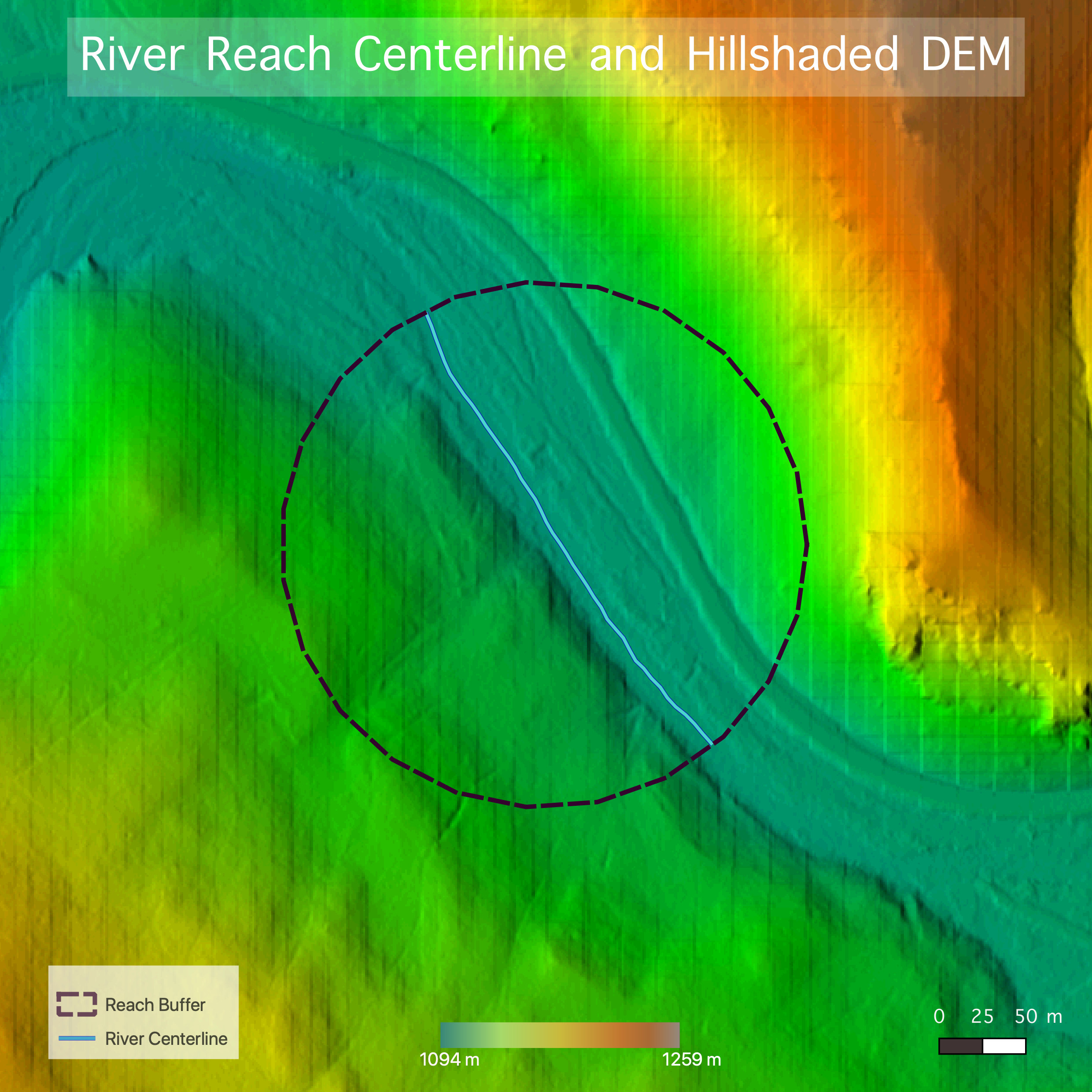
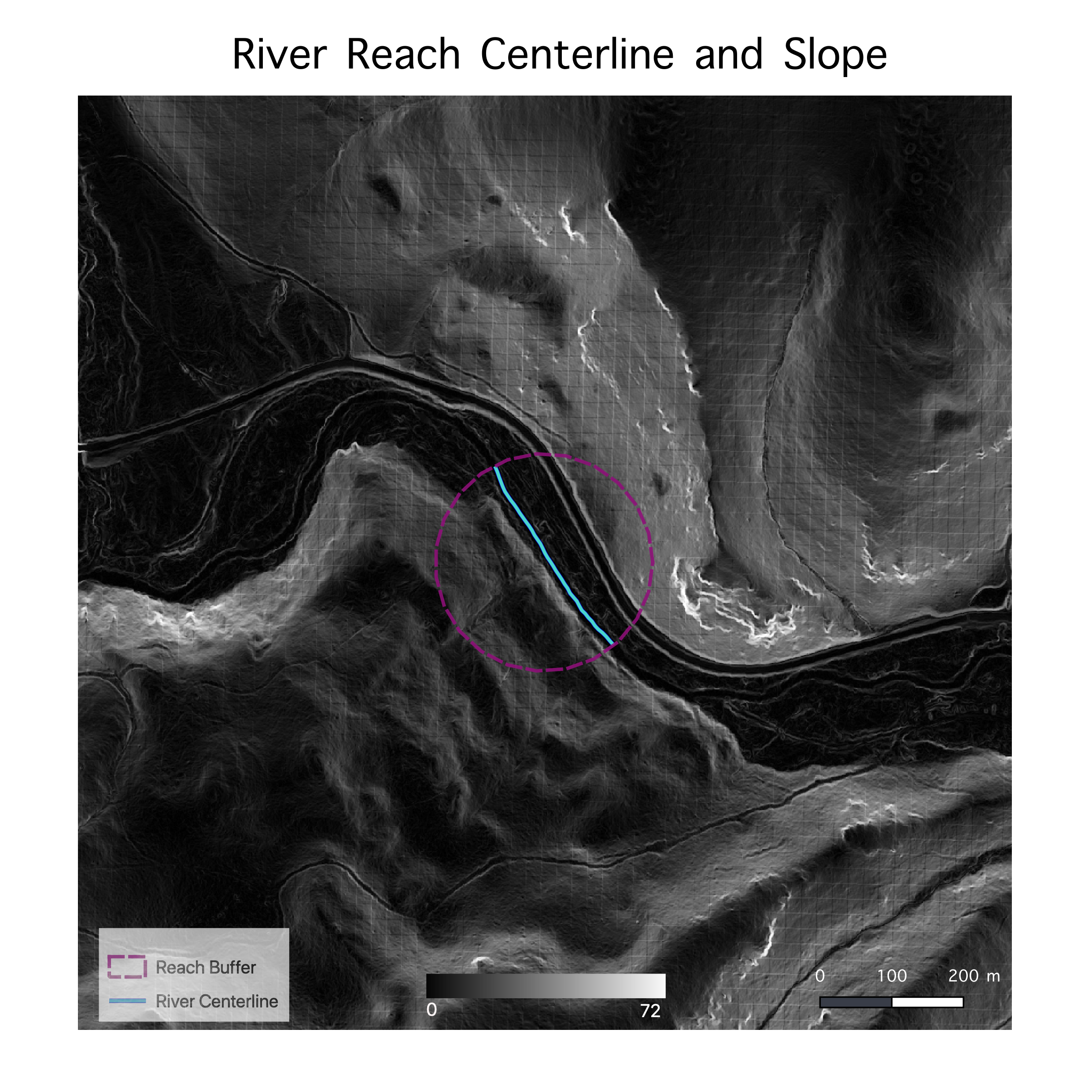 (Figs. 2a and 2b) Images of the shaded DEM (2a) and slope (2b) produced by the above model, shown with the reach buffer and river centerline.
We then digitized the banks three separate times, each time in a new vector map, and did the same for the valley edges. In each new layer, the banks or valley edges of the river were digitized as new vector lines at 1:1500 scale (Figs. 3a and 3b). Two of the digitizations for both the banks and the valley layers were done using the slope layer (Fig. 2b), and the third used a hillshaded DEM (Fig. 2a) as reference.
In order to find the centerlines (and centerline lengths) of the river and the valley, we used this model, also created by Joe Holler.
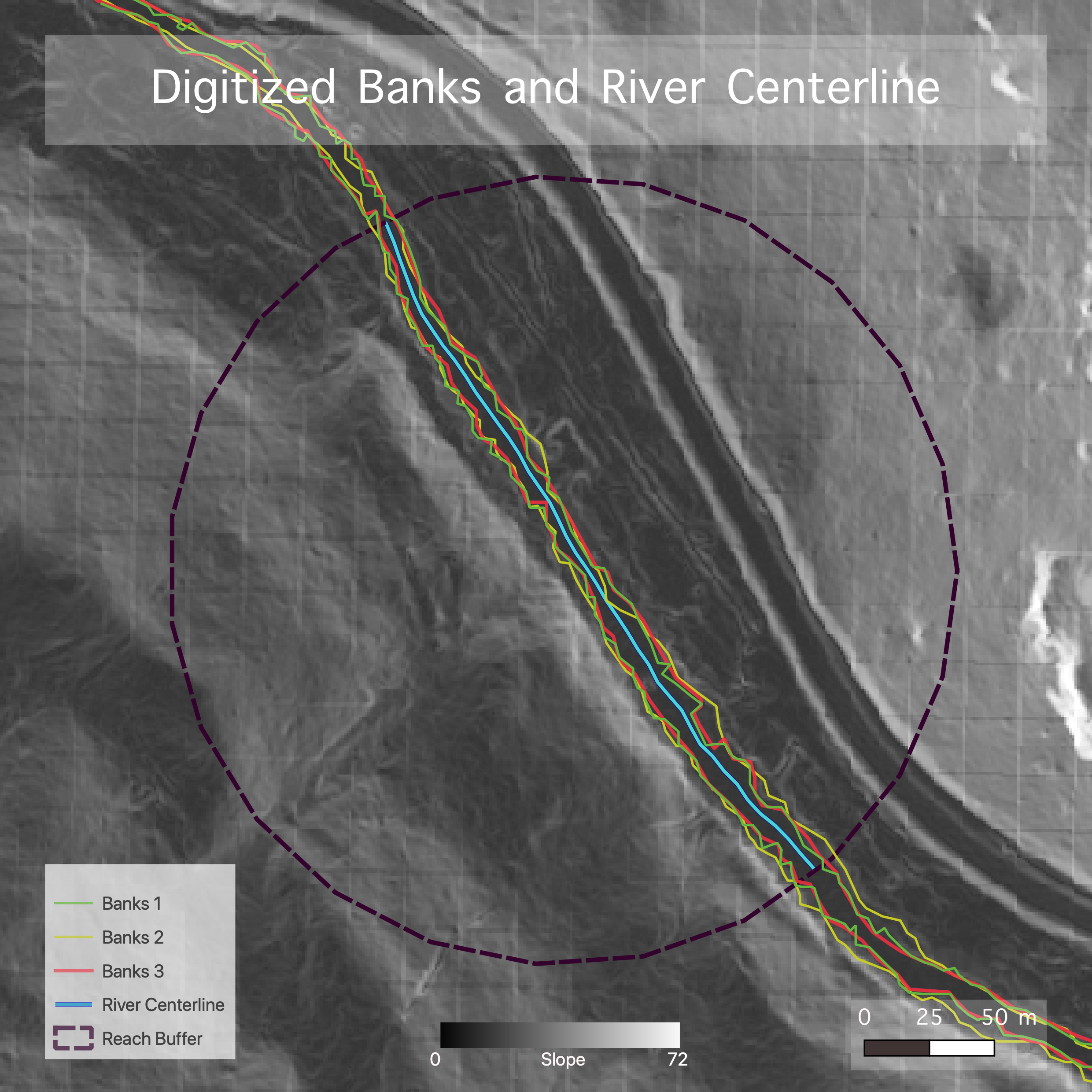
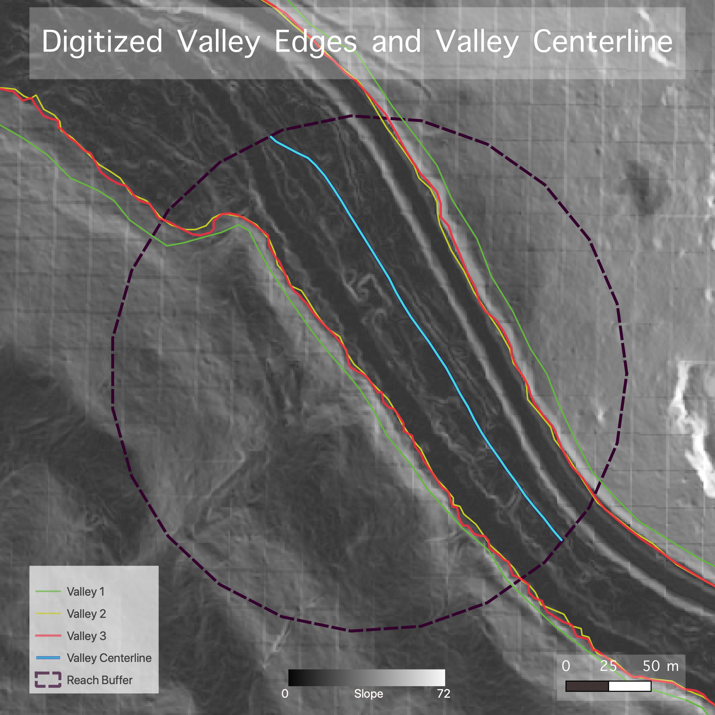 (Figs. 3a and 3b) Maps of the slope produced by the first model, shown with the digitized bank lines and bank centerlines (first map, 3a) and digitized valley edges and valley centerline (second map, 3b).
We then created the longitudinal profile of our river reach and extracted the profile as a series of longitudinal points in a textfile with the elevation data corresponding to the point coordinates. We also extracted the cross-sectional profile of a transect very near to the CHaMP point we had been assigned, and transformed that transect into a series of points, which we extracted, along with elevation data of the points, as a textfile. (Again, instructions can be found here.
Once we had the outputs for the centerlines of the rivers and valleys, we took the textfile data regarding the cross-sectional profile points and the longitudinal profile points into R. This script, created by Zach Hilgendorf, was used to extract a longitudinal profile and cross-sectional profile of the river reach using the data from the textfiles exported from GRASS. The script also calculated and plots the slope of the reach. However, the slope was calculated as an average of slopes between consecutive points along the transect, and due to digitizing errors (e.g. marking the slope as higher up the bank than it should have been) led to some of the slopes being far steeper than others. Therefore, the slope between the first point and the last point in the reach was manually calculated and compared to the average slope value.
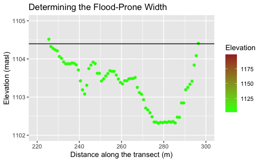
Finally, the R script plotted the cross-sectional profile with flood prone area demarkated by a black line (flood-prone area here defined as twice the bankfull depth).
We then classified our river using the RCS diagram provided by the EPA according to this criteria.
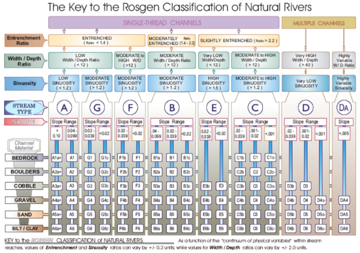 (Fig. 4) EPA rendition of the RCS classification process.
Level I classification was determined using entrenchment ratio, width/depth ratio, and sinuosity. Level II was determined using calculated slope value and channel material (taken from SubD50 attribute).
Replication Results
Table 1. Site Measurements (CHaMP_Data_MFJD Site ID from Site_x attribute: CBW05583-275954)
| Variable | Value | Source |
|---|---|---|
| Bankfull Width | 15.1702 m | BFWdth_AVG from CHaMP_Data_MFJD |
| Bankfull Average Depth | 0.4629 m | DpthBf_Avg from CHaMP_Data_MFJD |
| Bankfull Maximum Depth | 1.0406 m | DpthBF_Max from CHaMP_Data_MFJD |
| Valley Width | 73.85 m | R output from cross-sectional valley profile |
| Valley Depth | 2.1 m | R output from cross-sectional valley profile |
| Stream/River Length | 301.5354 m | GRASS layer banksLine |
| Valley Length | 296.413737 m | GRASS layer valleyLine |
| Median Channel Material Particle Diameter | 71 mm | SubD50 from CHaMP_Data_MFJD |
Table 2. Rosgen Level I Classification
| Criteria | Value |
|---|---|
| Entrenchment Ratio | 4.6143 |
| Width / Depth Ratio | 32.7720 |
| Sinuosity | 1.0173 |
| Level I Stream Type | C |
Table 3. Rosgen Level II Classification
| Criteria | Value |
|---|---|
| Slope | 0.0066833 |
| Channel Material | Cobble |
| Level II Stream Type | C3 |
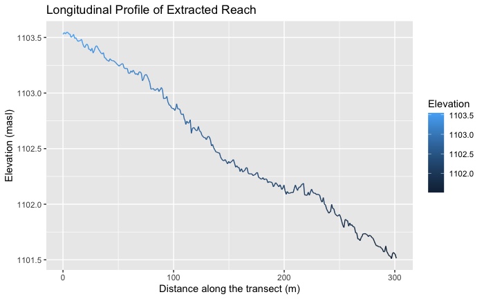 (Fig. 5) R output of longitudinal stream profile.
 (Fig. 6) R output of cross-sectional stream profile with 2x bankfull depth shown as black line.
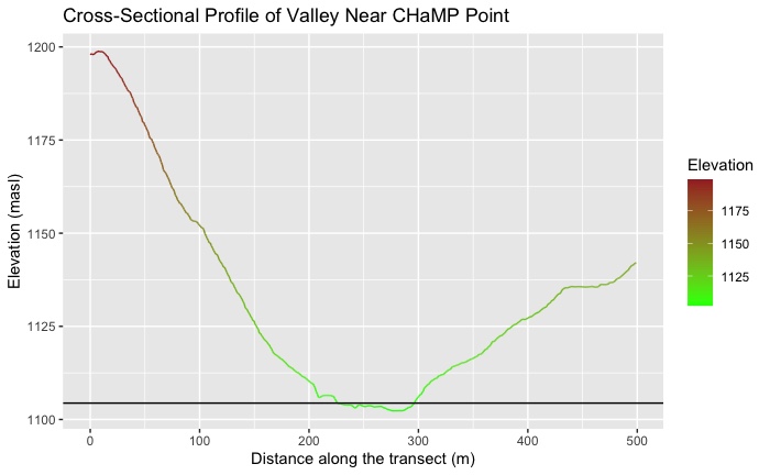
(Fig. 7) Zoomed in R output of cross-sectional valley profile with 2x bankfull depth shown as black line.
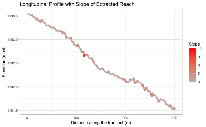 (Fig. 8) R output of longitudinal stream profile indicating slope changes between points.
Unplanned Deviations from the Protocol
The only deviation from the protocol was re-calculating slope as a general value from the start point to the end point of the longitudinal profile. In the original code, the slope value was calculated as the average slope value between each point derived from the reach centerline. Due to digitizing errors, there were some outliers of much higher elevation that were marked higher up the banks than they should have been, as can be seen in the longitudinal slope profile above (Fig. 8). This skewed the results of the slope average, resulting in a slope of 1.715. Re-calculating slope as the slope between the beginning and end points as Slope at Starting Point / Slope at End Point accounted for some of the digitizing uncertainty and yielded a much more credible value of 0.0066833 that aligns with the RCS. Additionally, it appears that there was some error in the digitization using one of the base layers that included a road running along the valley edge (Fig. 3b).
Results/ Discussion
Our results differed from those of Kasprak et al. (2016). The original study found that this river reach (CBW05583-275954) was of the type B3c, while our analysis led to the conclusion that this reach is type C3 (Table 3). Although the Level I classification is not the same (Table 2), the entrenchment ratio value seems to be the main factor that results in our classification being different from that of the original study (Table 2). There are several factors that may be causing this discrepancy. It is important to consider that we are introducing a great deal of uncertainty in this digitization process, no matter how carefully we attempted to pick out the banks and valley edges in this data (Figs. 2a and 2b). One factor that caused some inconsistencies in slope and potentially in the centerline calculations was that all digitization was done at 1:1500 scale. At that resolution, it was difficult to very accurately pick out and trace the banks of the river. Perhaps if there were a way to automate this digitization to ensure that it was based on clear, data-driven elevational differences, this would provide a solution to some of this uncertainty. The fact that this digitization was done by a novice instead of an expert in stream geomorphology also introduced uncertainty into this process.
Another potential driver of the difference in our results was the fact that we used different materials and methods than those in the original study. Like Kasprak et al. (2016), we used GIS to test the RCS. However, we used original models and code in the platforms GRASS and R, while they used the River Bathymetry Toolkit to determine the values of river classification criteria. In addition, our data differed from that used in Kasprak et al. (2016). Our study used Camp Creek LiDAR DEM data, which had a resolution of 1m x 1m. Conversely, Kasprak et al. (2016) used DEM data with 0.1m grid resolution. This difference in resolution is another potential source of uncertainty in our digitization process and in our slope calculations. There are also errors in our data, as evidenced in Fig. 2a by the vertical lines in the shaded DEM in Fig. 2a. We also did not have access to high-resolution topographic data nor to on-the-ground photographs of the site to check the accuracy or validity of our assessment, and did not “check” our results in that way. In addition, we used different methods to pick out our bankfull water surface, relying on the CHaMP data for average bankfull width rather than using the CHaMP Topo Toolbar to derive a bankfull water surface as Kasprak et al. (2016) did.
Aside from the entrenchment ratio, the sinuosity value is slightly lower than those of both B and C RCS stream types (typically >1.2, whereas our value was 1.0173 [Table 3]). The calculated sinuosity only aligns with that of an RCS Class A stream. This may be due to the approximated centerlines extrapolated from the digitized banks and valley edges losing some of the variability reflected in the banks. Additionally, although there is little temporal separation between our study and Kasprak et al. (2016), it is interesting to give some consideration here the impact of time on changes in fluvial form and behavior.
The width/depth ratio for this side, as well as the slope (as calculated between the highest and lowest points of the reach) and substrate material are very similar for the B3c and and C3 stream types. Our data regarding the width/depth and channel substrate come from the CHaMP data. However, our slope value came from the longitudinal profile created in GRASS and fits well within the confines of the stream classification given by Kasprak et al. (2016). This indicates that there was some similarity between our analysis and that of the original study.
Conclusions
In this case, the results of our analysis did not align with those of Kasprak et al. (2016). It is assumed that the RCS, which is based on quantitative metrics, should produce the same or very similar results in stream classification due to the nature of the variables upon which the classification is based. If this were a reproduction study, we would have had access to the same data and software platforms as those used in the original study. However, this was replication attempt and our data and methods differed from those used by the original study. There are many factors to which we may attribute the discrepancy between our results and those of Kasprak et al. (2016), as mentioned above. There were several instances in which we introduced uncertainty into our analysis (e.g. digitization process, lower resolution data), and these likely contributed to the difference in our classification. This study illustrates the importance of accounting for (or, at the very least, acknowledging) uncertainty in GIS analyses. We do not attempt to “explain away” the discrepancies between our analysis and the results of Kasprak et al. (2016), but considering the ways in which our analysis could be improved may help produce more reliable results that could be compared to those of the original study.
Data
- CHaMP_Data_MFJD from Columbia Habitat Monitoring Program
- John Day Watershed zipfile
- GRASS outputs (bank centerline, valley centerline, cross-sectional profile textfile, cross-sectional points textfile, longitudinal profile textfile and longitudinal points textfile)
- The metadata details are here
Models and R script
- Visualization GRASS Model (Made by Joe Holler)
- River and Valley Centerline GRASS Model (Made by Joe Holler)
- R Script (Written by Zach Hilgendorf)
References
-
Kasprak, A., N. Hough-Snee, T. Beechie, N. Bouwes, G. Brierley, R. Camp, K. Fryirs, H. Imaki, M. Jensen, G. O’Brien, D. Rosgen, and J. Wheaton. 2016. The Blurred Line between Form and Process: A Comparison of Stream Channel Classification Frameworks ed. J. A. Jones. PLOS ONE 11 (3):e0150293. https://dx.plos.org/10.1371/journal.pone.0150293.
-
Rosgen, D. L. in CATENA 22 (3):169–199. https://linkinghub.elsevier.com/retrieve/pii/0341816294900019.
Report Template References & License
This template was developed by Peter Kedron and Joseph Holler with funding support from HEGS-2049837. This template is an adaptation of the ReScience Article Template Developed by N.P Rougier, released under a GPL version 3 license and available here: https://github.com/ReScience/template. Copyright © Nicolas Rougier and coauthors. It also draws inspiration from the pre-registration protocol of the Open Science Framework and the replication studies of Camerer et al. (2016, 2018). See https://osf.io/pfdyw/ and https://osf.io/bzm54/
Camerer, C. F., A. Dreber, E. Forsell, T.-H. Ho, J. Huber, M. Johannesson, M. Kirchler, J. Almenberg, A. Altmejd, T. Chan, E. Heikensten, F. Holzmeister, T. Imai, S. Isaksson, G. Nave, T. Pfeiffer, M. Razen, and H. Wu. 2016. Evaluating replicability of laboratory experiments in economics. Science 351 (6280):1433–1436. https://www.sciencemag.org/lookup/doi/10.1126/science.aaf0918.
Camerer, C. F., A. Dreber, F. Holzmeister, T.-H. Ho, J. Huber, M. Johannesson, M. Kirchler, G. Nave, B. A. Nosek, T. Pfeiffer, A. Altmejd, N. Buttrick, T. Chan, Y. Chen, E. Forsell, A. Gampa, E. Heikensten, L. Hummer, T. Imai, S. Isaksson, D. Manfredi, J. Rose, E.-J. Wagenmakers, and H. Wu. 2018. Evaluating the replicability of social science experiments in Nature and Science between 2010 and 2015. Nature Human Behaviour 2 (9):637–644. http://www.nature.com/articles/s41562-018-0399-z.