Emma Clinton's Portfolio
Collection of Open Source GIScience Projects
Project maintained by emmaclinton Hosted on GitHub Pages — Theme by mattgraham
RP- Vulnerability modeling for sub-Saharan Africa
Original study by Malcomb, D. W., E. A. Weaver, and A. R. Krakowka. 2014. Vulnerability modeling for sub-Saharan Africa: An operationalized approach in Malawi. Applied Geography 48:17–30. DOI:10.1016/j.apgeog.2014.01.004
Replication Authors: Emma Clinton, Joseph Holler, Kufre Udoh, Open Source GIScience students of Fall 2019 and Spring 2021
Replication Materials Available at: emmaclinton.github.io
Created: 24 April 2021
Revised: 27 April 2021
Abstract
The original study is a multi-criteria analysis of vulnerability to Climate Change in Malawi, and is one of the earliest sub-national geographic models of climate change vulnerability for an African country. The study aims to be replicable, and had 40 citations in Google Scholar as of April 8, 2021.
Original Study Information
The study region is the country of Malawi. The spatial support of input data includes DHS survey points, Traditional Authority boundaries, and raster grids of flood risk (0.833 degree resolution) and drought exposure (0.416 degree resolution).
The original study was published without data or code, but has detailed narrative description of the methodology. The methods used are feasible for undergraduate students to implement following completion of one introductory GIS course. The study states that its data is available for replication in 23 African countries.
Data Description and Variables
Access and Assets Data: Demographic and Health Survey data are a product of the United States Agency for International Development (USAID). Variables contained in this dataset are used to represent adaptive capacity (access + assets) in Malcomb et al.’s (2014) study. These data come from survey questionnaires with large sample sizes. The DHS data used in our study were collected in 2010. In Malawi, the DHA data dates back as far as 1992, but data has not been collected consistently every year.
Each point in the household dataset represents a cluster of households, with each cluster corresponding to some form of census enumeration units, such as villages in rural areas or city blocks in urban areas DHS GPS Manual. This means that each household in each cluster has the same GPS data. This data is collected by trained USAID staff using GPS receivers. To preserve privacy, these points are then displaced randomly some distance from their origin, sometimes moved up to 2 km in urban areas or 5 km in more rural areas.
Missing data is a common occurrence in this dataset as a result of negligence or incorrect naming. However, according to the DHS GPS Manual, these issues are easily rectified and typically sites for which data does not exist are recollected. Sometimes, however, missing information is coded in as such or assigned a proxy location.
The DHS website acknowledges the high potential for inconsistent or incomplete data in such broad and expansive survey sets. Missing survey data (responses) are never estimated or made up; they are instead coded as a special response indicating the absence of data. As well, there are clear policies in place to ensure the data’s accuracy. More information about data validity can be found on the DHS’s Data Quality and Use site. In this analysis, we use the variables listed in Table 1 to determine the average adaptive capacity of each TA area. Data transformations are outlined below.
Metadata source: Burgert, C. R., Zachary, B., Colston, J. The DHS Program—Data. (2010). The DHS Program–USAID. Retrieved April 19, 2021, from https://dhsprogram.com/Data/) (file in metadata called DHS_GPS_Manual_English_A4_24May2013_DHSM9.pdf)
Table 1. DHS variables used in this analysis.
| Variable Code | Definition |
|---|---|
| HHID | “Case Identification” |
| HV001 | “Cluster number” |
| HV002 | “Household number” |
| HV246A | “Cattle own” |
| HV246D | “Goats own” |
| HV246E | “Sheep own” |
| HV246G | “Pigs own” |
| HV248 | “Number of sick people 18-59” |
| HV245 | “Hectares for agricultural land” |
| HV271 | “Wealth index factor score (5 decimals)” |
| HV251 | “Number of orphans and vulnerable children” |
| HV207 | “Has Radio” |
| HV243A | “Has a Mobile Telephone” |
| HV219 | “Sex of Head of Household” |
| HV226 | “Type of Cooking Fuel” |
| HV206 | “Has electricty” |
| HV204 | “Time to get to Water Source” |
Variable Transformations
- Eliminate households with null and/or missing values
- Join TA and LHZ ID data to the DHS clusters
- Eliminate NA values for livestock
- Sum counts of all different kinds of livestock into a single variable
- Apply weights to normalized indicator variables to get scores for each category (assets, access)
- Find the statistics of the capacity of each TA (min, max, mean, sd)
- Join ta_capacity to TAs based on ta_id
- Prepare breaks for mapping
- Class intervals based on capacity_2010 field
- Take the values and round them to 2 decimal places
- Put data in 4 classes based on break values
Livelihood Zones Data:
The livelihood zone (LHZ) data is created by aggregating general regions where similar crops are grown and similar ecological patterns exist. This data exists originally at the household level and was aggregated into Livelihood Zones. To construct the aggregation used for “Livelihood Sensitivity” in this analysis, we use these household points from the FEWSNet data that had previously been aggregated into livelihood zones.
The four Livelihood Sensitivity categories are 1) Percent of food from own farm (6%); 2) Percent of income from wage labor (6%); 3) Percent of income from cash crops (4%); and 4) Disaster coping strategy (4%). In the original R script, household data from the DHS survey was used as a proxy for the specific data points in the livelihood sensitivity analysis (transformation: Join with DHS clusters to apply LHZ FNID variables).
The LHZ data variables are outlined in Table 2. The four categories used to determine livelihood sensitivity were ranked from 1-5 based on percent rank values and then weighted using values taken from Malcomb et al. (2014).
Metadata source: Malawi Baseline Livelihood Profiles, Version 1* (September 2005). Made by Malawi National Vulnerability Assessment Committee in collaboration with the SADC FANR Vulnerability Assessment Committee (file in metadata called mw_baseline_rural_en_2005.pdf)
Table 2. Constructing livelihood sensitivity categories
| Livelihood Sensitivity Category (LSC) | Percent Contributing | How LSC was constructed |
|---|---|---|
| Percent of food from own farm | 6% | Sources of food: crops + livestock |
| Percent of income from wage labor | 6% | Sources of cash: labour etc. / total * 100 |
| Percent of income from cash crops | 4% | sources of cash (Crops): (tobacco + sugar + tea + coffee) + / total sources of cash * 100 |
| Disaster coping strategy | 4% | Self-employment & small business and trade: (firewood + sale of wild food + grass + mats + charcoal) / total sources of cash * 100 |
Physical Exposure Data: Flood Data: This dataset stems from work collected by multiple agencies and funneled into the PREVIEW Global Risk Data Platform, “an effort to share spatial information on global risk from natural hazards.” The dataset was designed by UNEP/GRID-Europe for the Global Assessment Report on Risk Reduction (GAR), using global data. A flood estimation value is assigned via an index of 1 (low) to 5 (extreme). The resolution of this data is 0.833 degrees.
Drought Data:This dataset uses the Standardized Precipitation Index to measure annual drought exposure across the globe. The Standardized Precipitation Index draws on data from a “global monthly gridded precipitation dataset” from the University of East Anglia’s Climatic Research Unit, and was modeled in GIS using methodology from Brad Lyon at Columbia University. The dataset draws on 2010 population information from the LandScanTM Global Population Database at the Oak Ridge National Laboratory. Drought exposure is reported as the expected average annual (2010) population exposed. The data were compiled by UNEP/GRID-Europe for the Global Assessment Report on Risk Reduction (GAR). The data use the WGS 1984 datum, span the years 1980-2001, and are reported in raster format with spatial resolution 1/24 degree x 1/24 degree.
Metadata source: Global Risk Data Platform: Data-Download. (2013). Global Risk Data Platform.
Drought: Physical exposition to droughts events 1980-2001 https://preview.grid.unep.ch/index.php?preview=data&events=droughts&evcat=4&lang=eng
Global estimated risk index for flood hazard https://preview.grid.unep.ch/index.php?preview=data&events=floods&evcat=5&lang=eng
Variable Transformations
- Load in UNEP raster
- Set CRS for drought to EPSG:4326
- Set CRS for flood to EPSG:4326 1.Reproject, clip, and resample based on bounding box (dimensions: xmin = 35.9166666666658188, xmax = 32.6666666666658330, ymin = -9.3333333333336554, ymax = -17.0833333333336270) and resolution of blank raster we created: resolution is 1/24 degree x 1/24 degree
- Use bilinear resampling for drought to average continuous population exposure values
- Use nearest-neighbor resampling for flood risk to preserve integer values
Malawi Traditional Authorities: Source: Download GADM data (version 2.8). (2018). Database of Global Administrative Areas. https://gadm.org/download_country_v2.html
Major Lakes: Source: http://www.masdap.mw/ Taken from OSM Variable Transformations: used in EA variable to classify major lakes as such in final representation
Analytical Specification
The original study was conducted using ArcGIS and STATA, but does not state which versions of these software were used. The replication study will use R.
Materials and Procedure
The steps outlined below mirror the steps used in the R Code for this project.
Process Adaptive Capacity
- Bring in DHS Data [Households Level] (vector)
- Bring in TA (Traditional Authority boundaries) and LHZ (livelihood zones) data
- Get rid of unsuitable households (eliminate NULL and/or missing values)
- Join TA and LHZ ID data to the DHS clusters
- Pre-process the livestock data Filter for NA livestock data Update livestock data (summing different kinds)
- FIELD CALCULATOR: Normalize each indicator variable and rescale from 1-5 (real numbers) based on percent rank
- FIELD CALCULATOR / ADD FIELD: Apply weights to normalized indicator variables to get scores for each category (assets, access)
- SUMMARIZE/AGGREGATE: find the stats of the capacity of each TA (min, max, mean, sd)
- Join ta_capacity to TA based on ta_id (Multiply by 20–meaningless??) I have a question about this (so do I) ln.216
- Prepare breaks for mapping Class intervals based on capacity_2010 field Take the values and round them to 2 decimal places Put data in 4 classes based on break values
- Save the adaptive capacity scores
Process Livelihood Sensitivity
- Load in LHZ geometries into R
- Join LHZ sensitivity data into R code
- Read in processed LHZ dataset
- Join the data to the LHZ geometries
- Put LHZ data into quintiles
- Calculate capacity score based on values in Malcomb et al. (2014)
Process Physical Exposure
- Load in UNEP rasterSet CRS for drought
- Set CRS for flood
- Clean and reproject rasters
- Create a bounding box at extent of Malawi Where does this info come from
- For Drought: use bilinear to avg continuous population exposure values
- For Flood: use nearest neighbor to preserve integer values
- CLIP the traditional authorities with the LHZs to cut out the lake
- RASTERIZE the ta_capacity data with pixel data corresponding to capacity_2010 field
- RASTERIZE the livelihood sensitivity score with pixel data corresponding to capacity_2010 field
Raster Calculations
- Create a mask
- Reclassify the flood layer (quintiles, currently binary)
- Reclassify the drought values (quantile [from 0 - 1 in intervals of 0.2 =5])
- AGGREGATE: Create final vulnerability layer using environmental vulnerability score and ta_capacity.
We then georeferenced maps from the original study using QGIS in order to compare the results generated by our R script to those found in Malcomb et al. (2014). We ran a Spearman’s Rho correlation test between the two maps of Figs. 4 and 5 to determine the differences in results.
Unplanned Deviations from the Protocol
Our first pass at creating a workflow before seeing the data outlined several areas of uncertainty. For instance, we were unsure of at what level of organization the DHS data came in (household level, village level, or district level). We were also unsure about (and remain unsure about) the factors outlined below, which are ultimate sources of uncertainty in our replication analysis.
In this protocol, it was unclear how exactly the livelihood zones data were divided into the four categories of livelihood sensitivity. This is a large source of uncertainty in our analysis. In addition, the original study states that it broke the data into quintiles by assigning values of 0-5 to the data. This would actually result in six classes, or sextiles. We decided to use quintiles and assigned values of 1-5 when normalizing our data. It is also unclear how binary data in the original study was normalized on a 1-5 scale. For binary variables (e.g. sex), we assigned a value of 1 to the presumed lower-risk option (e.g. male) and a value of 2 to the higher-risk (e.g. female).
It was also unclear when data were aggregated to the TA level—was this done before or after the data scores were normalized and weighted in the original study? We decided to aggregate after the data had been normalized and weighted.
Discussion
Our replication analysis yielded slightly different results than those generated in the original study. Fig. 1 shows the results of our replication analysis in terms of access and assets in 2010 on the Traditional Authority level of organization (represented by Fig. 4 in the original study). Fig. 2 shows the difference between our results and those generated by Malcomb et al. (2014). This difference was calculated by subtracting values found in Malcomb et al. (2014) from the results of our study.
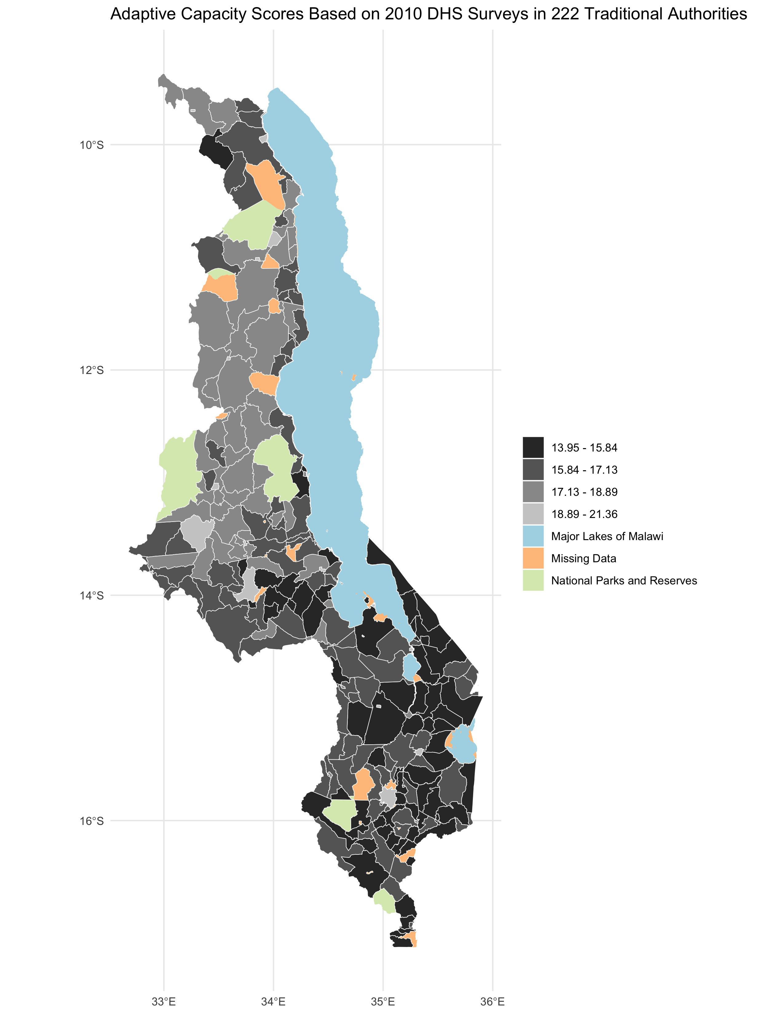 (Fig. 1) Access and assets (adaptive capacity) scores from our results.
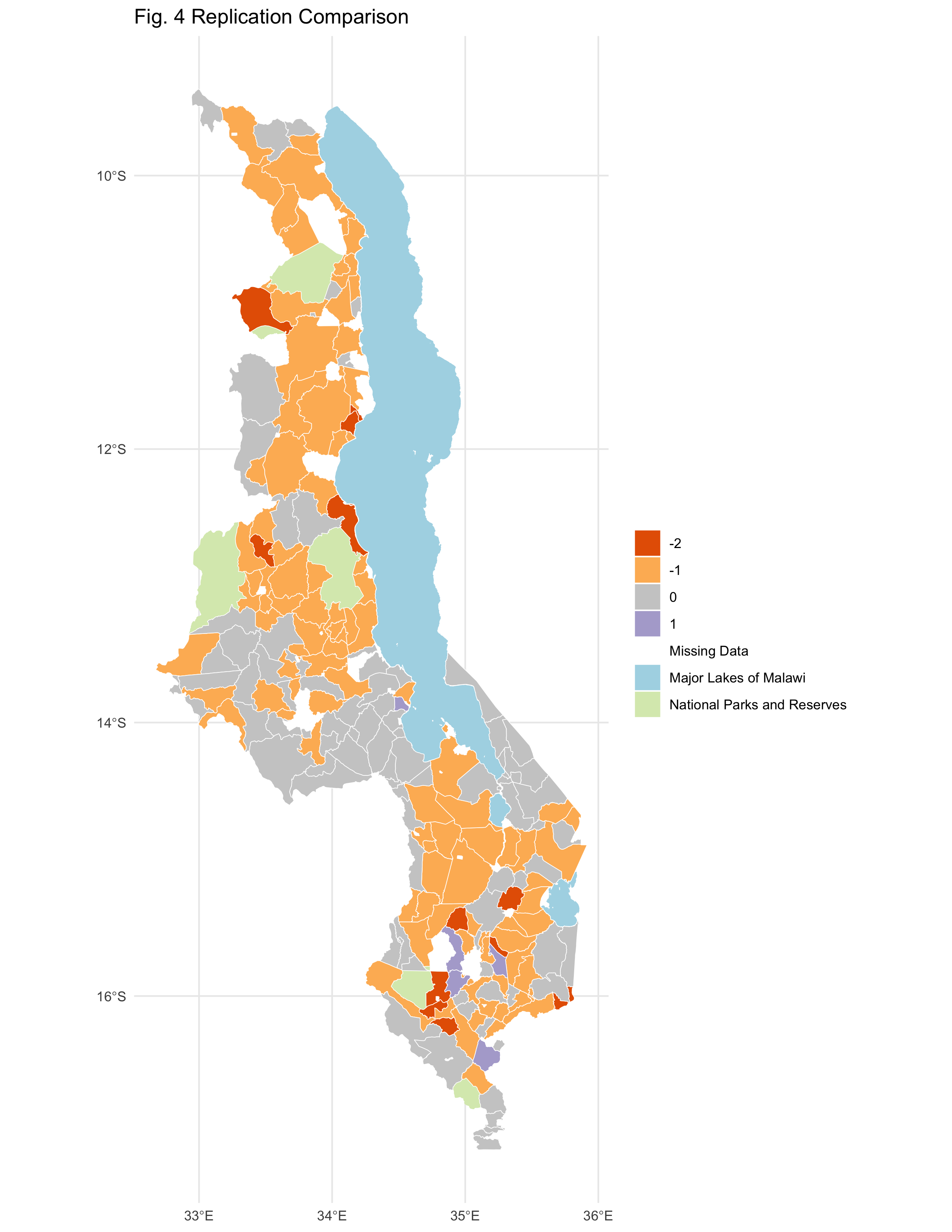 (Fig. 2) Difference in access and assets (adaptive capacity) scores (difference = reproduction score - original study score).
There are some differences between the two. Compared to Malcomb et al. (2014), our analysis seems to have generally provided lower adaptive capacity values than those in the original study. This may be due to a modification made to the code in which a line multiplying capacity values by 20 to make them more similar to the values of Malcomb et al. (20140 was removed. However, it may also be due to the sources of uncertainty outlined above: particularly the organization into quintiles and the uncertainty surrounding the timing of aggregation to the TA level. However, as indicated in Table 3, the rho value is relatively close to 1, indicating a positive correlation between the values of the two maps.
Table 3. Spearman’s rho correlation test results. (rho = 0.7856613). The results of the original study are shown on the x axis (columns), while the results of the reproduction are shown on the y axis (rows).
| 1 | 2 | 3 | 4 | |
|---|---|---|---|---|
| 1 | 34 | 5 | 0 | 0 |
| 2 | 25 | 25 | 0 | 0 |
| 3 | 5 | 43 | 20 | 0 |
| 4 | 0 | 7 | 27 | 5 |
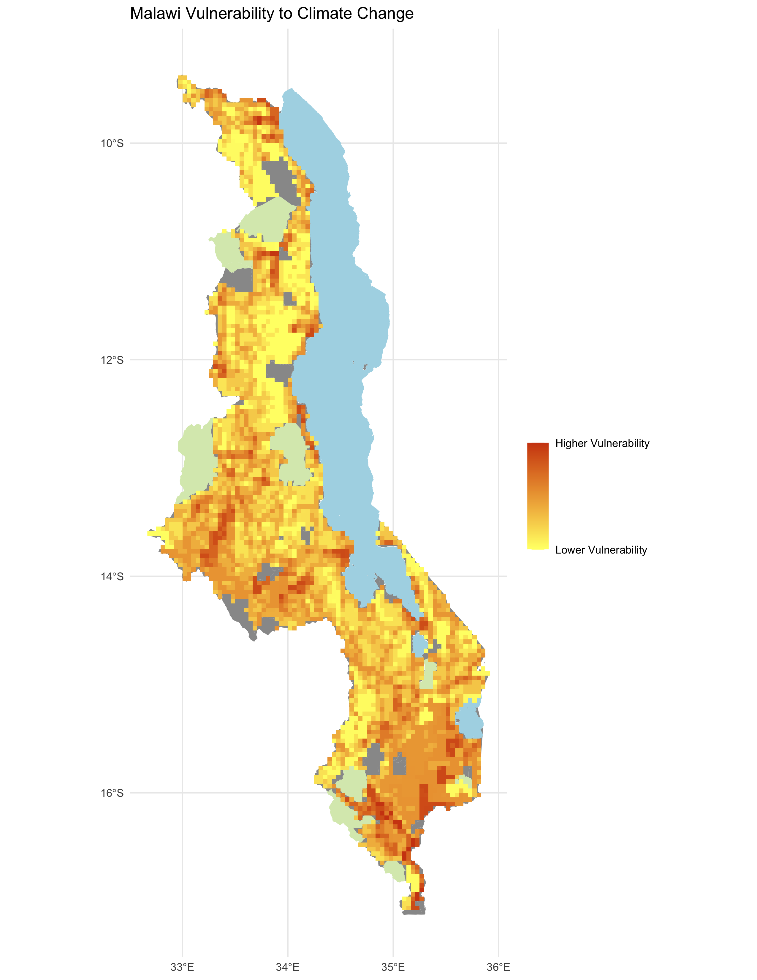 (Fig. 3) Final vulnerability score from our results.
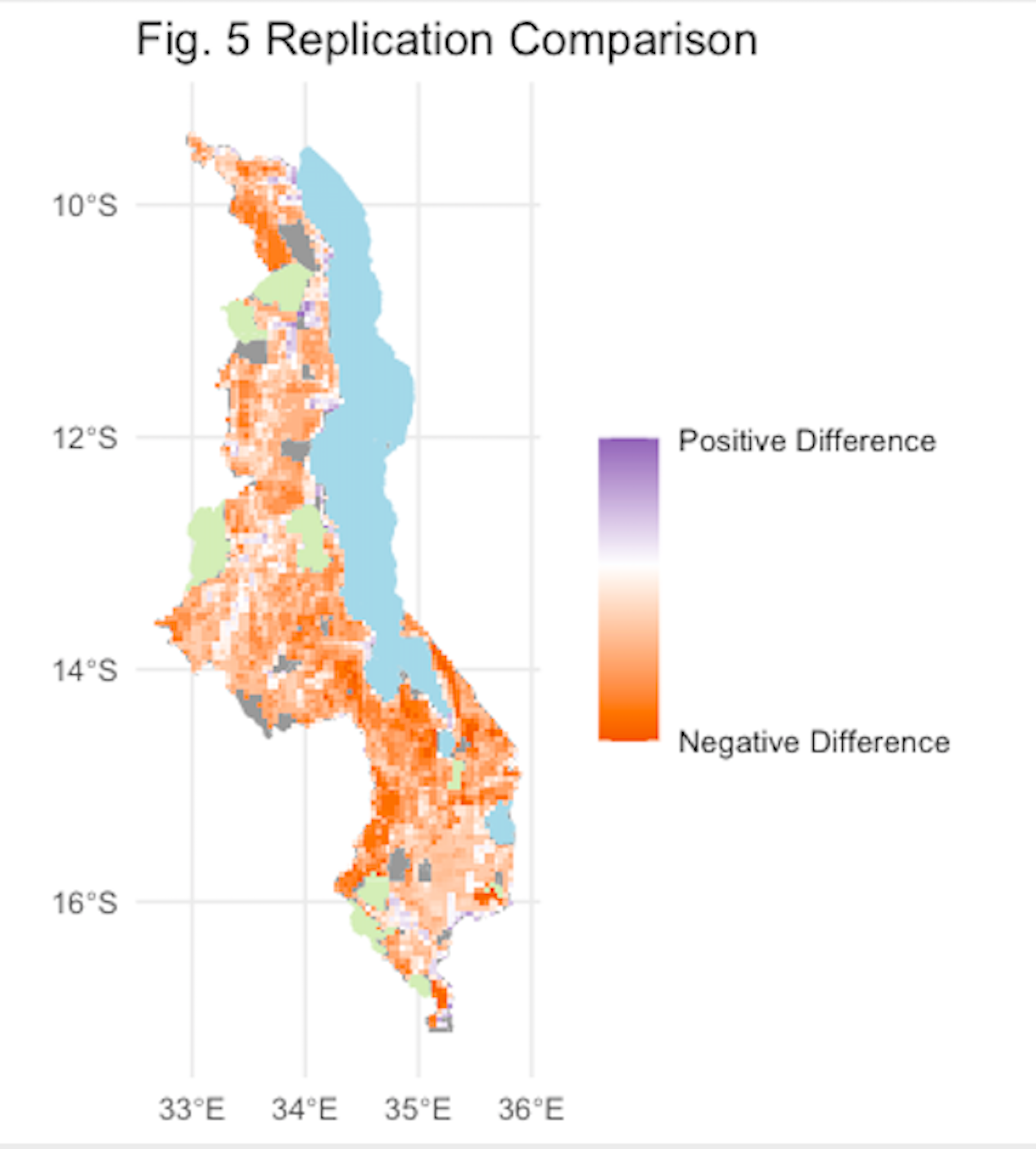 (Fig. 4) Final vulnerability score comparison between our results and those of the original study (difference = reproduction score - original score).
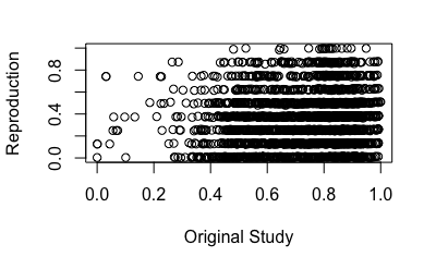
(Fig. 5) Final vulnerability score comparison between our results and those of the original study (difference = reproduction score - original score) in the form of a scatterplot (rho = 0.1859791).
The final vulnerability map (equivalent to Fig. 5 in Malcomb et al. [2014]) exhibited more difference than that seen in Fig. 4. Again, our analysis seems more likely to yield lower vulnerability values than the original. The Spearman’s correlation test yielded rho = 0.1859791, indicating low correlation between the values on the original and reproduction map. This may be due to the lack of clarity on how the variables corresponding to livelihood sensitivity; however, it appears that the values in the scatterplot are oddly discretized. It is possible that this is due to some earlier classification of the data or some lack of decimal precision that caused the values to appear more similar to one another than they otherwise might have been. For a view of the correct scatterplot, look here (credits to Maja Cannavo). There was substantial opportunity for variation in interpretation of the original methods in this section of the study. It is possible that our values are very different from those assigned by Malcomb et al. (2014) because there is no way to check that the way we calculated the variables in Table 2 parallels the calculations of the original authors.
Ultimately, we did not have the code used by the original authors when they carried out this study. This would not have been as much of a problem if the methods had been more explicit. However, this lack of code, combined with the fact that the methods were incompletely documented, means that there was a great deal of “room for interpretation” involved in our attempt to reproduce their results, even with 100% of the data used in the original study. Any discrepancies in our data are likely due to practical errors.
With that being said, there is also a great deal of uncertainty involved in the original study itself. Tate (2013) details a framework of uncertainty in vulnerability modeling. When Malcomb et al. (2014) is compared to this framework, there are several possible sources of subjectivity/uncertainty involved. For instance, the indicators of uncertainty used in this study were mostly normative (relying on expert opinion) or practical (meaning that the data available for use were used; this is interesting because it is likely that the experts interviewed for opinions were involved in the generation of a great deal of this data).
The normalization process was standardized for all variables but highly dependent on the data value ranges and was not very applicable to binary variables. The weighting of these variables was also normative, making it a subjective process of value judgement. In addition, the data were aggregated in an additive manner at the end of the study to generate a final vulnerability value. This is logical but means that if an area has a very high vulnerability value in one category but a very low value in another, the difference between the two is cancelled out and that high vulnerability is masked.
Additionally, the study makes no mention of uncertainty analysis, sensitivity analysis, or validation, meaning that areas where the model are most and least reliable are not highlighted in the results (Tate, 2013).
Conclusion
The fact that our final vulnerability values correlated only weakly with those of the original study is very telling. This reproduction analysis is an excellent example of why it is imperative to provide explicit methodology (and, preferably, access to code) when publishing academic work. This is especially important when publishing work with broad socioeconomic and social and environmental justice implications like climate vulnerability analyses.
It is also important to acknowledge the inherent sources of uncertainty in the original study (mentioned above) introduce subjectivity into this work, meaning that conclusions are drawn and resources allotted based on potentially biased or incomplete sources of information.
There is potential for future research on multiple fronts. It would be beneficial to try and recreate the original results from the original code or by acquiring more thoroughly documented methods. Another possibility would be performing an uncertainty analysis on our methods to determine the impacts of our modeling decisions on the uncertainty of our model.
Acknowledgements/Collaborations
I would like to thank my lab group—Drew An-Pham, Maja Cannavo, Jacob Freedman, Nick Nonnenmacher, and Alitzel Villanueva—for all of their assistance with designing and updating our workflow, assistance with coding quirks, and collaborative compilation of description of data sources, variables, and variable transformations. I would also like to thank Vincent Falardeau for supplementing code for Fig. 2.
References
Malcomb, D. W., E. A. Weaver, and A. R. Krakowka. 2014. Vulnerability modeling for sub-Saharan Africa: An operationalized approach in Malawi. Applied Geography 48:17–30. DOI:10.1016/j.apgeog.2014.01.004
Tate, E. 2013. Uncertainty Analysis for a Social Vulnerability Index. Annals of the Association of American Geographers 103 (3):526–543. doi:10.1080/00045608.2012.700616.
Report Template References & License
This template was developed by Peter Kedron and Joseph Holler with funding support from HEGS-2049837. This template is an adaptation of the ReScience Article Template Developed by N.P Rougier, released under a GPL version 3 license and available here: https://github.com/ReScience/template. Copyright © Nicolas Rougier and coauthors. It also draws inspiration from the pre-registration protocol of the Open Science Framework and the replication studies of Camerer et al. (2016, 2018). See https://osf.io/pfdyw/ and https://osf.io/bzm54/
Camerer, C. F., A. Dreber, E. Forsell, T.-H. Ho, J. Huber, M. Johannesson, M. Kirchler, J. Almenberg, A. Altmejd, T. Chan, E. Heikensten, F. Holzmeister, T. Imai, S. Isaksson, G. Nave, T. Pfeiffer, M. Razen, and H. Wu. 2016. Evaluating replicability of laboratory experiments in economics. Science 351 (6280):1433–1436. https://www.sciencemag.org/lookup/doi/10.1126/science.aaf0918.
Camerer, C. F., A. Dreber, F. Holzmeister, T.-H. Ho, J. Huber, M. Johannesson, M. Kirchler, G. Nave, B. A. Nosek, T. Pfeiffer, A. Altmejd, N. Buttrick, T. Chan, Y. Chen, E. Forsell, A. Gampa, E. Heikensten, L. Hummer, T. Imai, S. Isaksson, D. Manfredi, J. Rose, E.-J. Wagenmakers, and H. Wu. 2018. Evaluating the replicability of social science experiments in Nature and Science between 2010 and 2015. Nature Human Behaviour 2 (9):637–644. http://www.nature.com/articles/s41562-018-0399-z.